Interpolate a meridional section of CROCO outputs to regular depths

This notebook, we show:

• how to compute the depths from s-coordinates,

• how to easily find the name of variables and coordinates,

• how to interpolate a 3D field with varying depths to regular depths.

Inits

Import needed modules.

import numpy as np
import xarray as xr
import matplotlib.pyplot as plt
import cmocean
import xoa
from xoa.regrid import regrid1d

xr.set_options(display_style="text");

<xarray.core.options.set_options at 0x7f45a69d01f0>

Register the decode_sigma accessor.

xoa.register_accessors(decode_sigma=True)

The xoa accessor is also registered by default, and give access to most of the fonctionalities of the other accessors.

Read the model

This sample is a meridional extraction of a full 3D CROCO output.

ds = xoa.open_data_sample("croco.south-africa.meridional.nc")
ds

<xarray.Dataset>
Dimensions:     (auxil: 4, eta_rho: 56, eta_v: 55, s_rho: 32, s_w: 33, time: 1, xi_rho: 1, xi_u: 1)
Coordinates: (12/13)
  * eta_rho     (eta_rho) float32 6.0 7.0 8.0 9.0 10.0 ... 58.0 59.0 60.0 61.0
  * eta_v       (eta_v) float32 6.5 7.5 8.5 9.5 10.5 ... 57.5 58.5 59.5 60.5
    lat_rho     (eta_rho, xi_rho) float32 ...
    lat_u       (eta_rho, xi_u) float32 ...
    lat_v       (eta_v, xi_rho) float32 ...
    lon_rho     (eta_rho, xi_rho) float32 ...
    ...          ...
    lon_v       (eta_v, xi_rho) float32 ...
  * s_rho       (s_rho) float32 -0.9844 -0.9531 -0.9219 ... -0.04688 -0.01562
  * s_w         (s_w) float32 -1.0 -0.9688 -0.9375 ... -0.0625 -0.03125 0.0
  * time        (time) float64 2.592e+06
  * xi_rho      (xi_rho) float32 131.0
  * xi_u        (xi_u) float32 131.5
Dimensions without coordinates: auxil
Data variables: (12/23)
    AKt         (time, s_w, eta_rho, xi_rho) float32 ...
    Cs_r        (s_rho) float32 ...
    Cs_w        (s_w) float32 ...
    Vtransform  float32 ...
    angle       (eta_rho, xi_rho) float32 ...
    el          float32 ...
    ...          ...
    time_step   (time, auxil) int32 ...
    u           (time, s_rho, eta_rho, xi_u) float32 ...
    v           (time, s_rho, eta_v, xi_rho) float32 ...
    w           (time, s_rho, eta_rho, xi_rho) float32 ...
    xl          float32 ...
    zeta        (time, eta_rho, xi_rho) float32 ...
Attributes: (12/57)
    type:           ROMS history file
    title:          BENGUELA TEST MODEL
    date:
    rst_file:       CROCO_FILES/croco_rst.nc
    his_file:       CROCO_FILES/croco_his.nc
    avg_file:       CROCO_FILES/croco_avg.nc
    ...             ...
    v_sponge:       0.0
    sponge_expl:    Sponge parameters : extent (m) & viscosity (m2.s-1)
    SRCS:           main.F step.F read_inp.F timers_roms.F init_scalars.F ini...
    CPP-options:    REGIONAL BENGUELA_VHR MPI OBC_EAST OBC_WEST OBC_NORTH OBC...
    history:        Tue Mar 31 16:26:24 2020: ncks -O -d time,30 -d xi_rho,13...
    NCO:            4.4.2

Compute depths from s-coordinates

Decode the dataset according to the CF conventions:

1. Find sigma terms

2. Compute depths

3. Assign depths as coordinates

Note that the decode_sigma accessor calls the xoa.sigma.decode_cf_sigma function.

ds = ds.decode_sigma()
ds.depth

<xarray.DataArray 'depth' (time: 1, s_rho: 32, eta_rho: 56, xi_rho: 1)>
array([[[[-4.4787710e+03],
         [-4.4534194e+03],
         [-4.4333271e+03],
         ...,
         [-7.3894226e+01],
         [-7.3414513e+01],
         [-7.3409134e+01]],

        [[-4.1099888e+03],
         [-4.0867766e+03],
         [-4.0683792e+03],
         ...,
         [-7.0494987e+01],
         [-7.0042336e+01],
         [-7.0037262e+01]],

        [[-3.7039980e+03],
         [-3.6831455e+03],
         [-3.6666174e+03],
         ...,
...
         ...,
         [-4.2952929e+00],
         [-4.2748423e+00],
         [-4.2746129e+00]],

        [[-1.0079492e+01],
         [-1.0048058e+01],
         [-1.0017785e+01],
         ...,
         [-2.5738845e+00],
         [-2.5616508e+00],
         [-2.5615137e+00]],

        [[-3.1787627e+00],
         [-3.1540668e+00],
         [-3.1291361e+00],
         ...,
         [-8.5690212e-01],
         [-8.5283607e-01],
         [-8.5279047e-01]]]], dtype=float32)
Coordinates:
  * eta_rho  (eta_rho) float32 6.0 7.0 8.0 9.0 10.0 ... 57.0 58.0 59.0 60.0 61.0
    lat_rho  (eta_rho, xi_rho) float32 ...
    lon_rho  (eta_rho, xi_rho) float32 ...
  * s_rho    (s_rho) float32 -0.9844 -0.9531 -0.9219 ... -0.04688 -0.01562
  * time     (time) float64 2.592e+06
  * xi_rho   (xi_rho) float32 131.0
    depth    (time, s_rho, eta_rho, xi_rho) float32 -4.479e+03 ... -0.8528
Attributes:
    standard_name:  ocean_layer_depth
    long_name:      Depth
    units:          m

Find coordinate names from CF conventions

The depth was assigned as coordinates at the previous stage. We use the xoa data array accessor to easily access the temperature, latitude and depth arrays.

temp = ds.xoa.temp.squeeze()
lat_name = temp.xoa.lat.name

Interpolate at regular depths

We interpolate the temperature array from irregular to regular depths.

Let’s create the output depths.

depth = xr.DataArray(np.linspace(ds.depth.min(), ds.depth.max(), 100),
                     name="depth", dims="depth")

Let’s interpolate the temperature.

tempz = regrid1d(temp, depth)

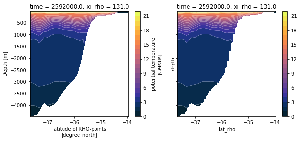
Plots

Make a basic comparison plots.

fig, axs = plt.subplots(ncols=2, sharex=True, sharey=True, figsize=(10, 4))
kw = dict(levels=np.arange(0, 23))
temp.plot.contourf(lat_name, "depth", cmap="cmo.thermal", ax=axs[0], **kw)
temp.plot.contour(lat_name, "depth", colors='w', linewidths=.3, ax=axs[0], **kw)
tempz.plot.contourf(lat_name, "depth", cmap="cmo.thermal", ax=axs[1], **kw)
tempz.plot.contour(lat_name, "depth", colors='w', linewidths=.3, ax=axs[1], **kw);

<matplotlib.contour.QuadContourSet at 0x7f45977f7490>

Et voilà!