Compare Mercator to ARGO

In this notebook, we show:

• how to easily rename variables and coordinates in an ARGO and a Mercator datasets,

• how to plot a T-S diagram,

• how to stack geographical coordinates,

• how to compute a geographical distance between two datasets with coordinates,

• how to interpolate a vertical profile with different methods.

Initialisations

import xarray as xr
import matplotlib as mpl
import matplotlib.pyplot as plt
import cartopy.crs as ccrs
import gsw
import cmocean

import xoa
import xoa.grid as xgrid
import xoa.regrid as xregrid
import xoa.meta as xmeta
import xoa.coords as xcoords
import xoa.geo as xgeo
import xoa.plot as xplot

mpl.rc("axes", grid=True)
xr.set_options(display_style="text")

<xarray.core.options.set_options object at 0x75968fb65590>

Register the xoa accessors :

xoa.register_accessors()

Register the Mercator and ARGO naming specifications

mercator_cfg = xoa.get_meta_config_file("mercator")
argo_cfg = xoa.get_meta_config_file("argo")
xmeta.register_meta_specs(mercator_cfg)
xmeta.register_meta_specs(argo_cfg)

Here is what these CF specifications contain

with open(mercator_cfg) as f:
    print(f.read())
with open(argo_cfg) as f:
    print(f.read())

[register]
name=mercator
    [[attrs]]
    source=IBI-MFC*
[data_vars]
    [[temp]]
    name=thetao
    [[sal]]
    name=so
    [[u]]
    name=uo
    [[v]]
    name=vo
    [[ssh]]
    name=zos



[register]
name=argo
    [[attrs]]
    DATA_ID=ARGO
    source=drifting subsurface profiling float
[sglocator]
name_format=False
[data_vars]
    [[temp]]
    name=TEMP
    search_order=n
    [[temp_adjusted]]
    name=TEMP_ADJUSTED
    search_order=n
    [[sal]]
    name=PSAL
    search_order=n
    [[sal_adjusted]]
    name=PSAL_ADJUSTED
    search_order=n
    [[pres]]
    name=PRES
    search_order=n
    [[pres_adjusted]]
    search_order=n
    name=PRES_ADJUSTED
[coords]
    [[lon]]
    name=LONGITUDE
    [[lat]]
    name=LATITUDE
    [[level]]
    name=N_LEVELS
    [[time]]
    name=TIME

Read and decode the datasets

ARGO profiles

The ARGO data were downloaded with the argopy package with a piece of code close to the following:

from argopy import DataFetcher
adf = DataFetcher().float(7900573)
ds = adf.to_xarray().argo.point2profile().isel(N_PROF=slice(-10, None))
ds.to_netcdf("argo-7900573.nc")

Here is the web page of this float: https://fleetmonitoring.euro-argo.eu/float/7900573

ds_argo = xoa.open_data_sample("OBS/ARGO/argo-7900573.nc")

We decode the names to make them more generic thanks to the CF specifications and select only the variables of interest.

ds_argo = ds_argo.xoa.decode()[["temp", "sal", "pres"]]

We compute depths with the gsw package and assign them as coordinates of the ARGO dataset.

alat = ds_argo.lat.broadcast_like(ds_argo.pres)
adepth = gsw.z_from_p(ds_argo.pres, alat)
adepth = adepth.where(adepth.notnull(), adepth.min())
adepth.attrs.update({"long_name": "Depth", "units": "m"})
ds_argo = ds_argo.assign_coords(depth=adepth)
ds_argo = ds_argo.isel(level=slice(None, None, -1))
ds_argo = ds_argo.set_index(N_PROF="time").rename(N_PROF="time")

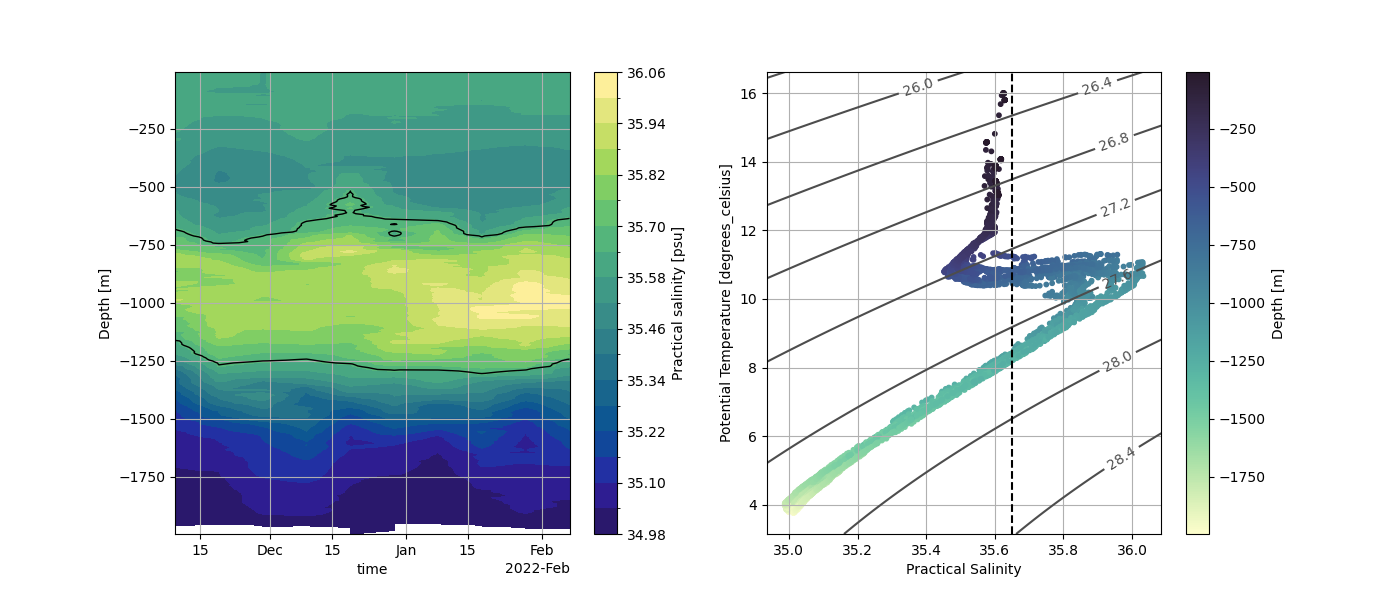
Quick plot of the salinity that highligths the mediterranean water.

fig, axs = plt.subplots(ncols=2, figsize=(14, 6))
ds_argo.sal.plot.contourf("time", "depth", cmap="cmo.haline", levels=20, ax=axs[0])
ds_argo.sal.plot.contour("time", "depth", levels=[35.65], linewidths=1, colors="k", ax=axs[0])
xplot.plot_ts(
    ds_argo.temp,
    ds_argo.sal,
    potential=False,
    scatter_c=ds_argo.depth,
    scatter_cmap="cmo.deep",
    axes=axs[1],
)
axs[1].axvline(x=35.65, ls="--", color="k")

/home/docs/checkouts/readthedocs.org/user_builds/xoa/conda/v2026.2.0/lib/python3.14/site-packages/xarray/plot/accessor.py:663: FutureWarning: Using positional arguments is deprecated for plot methods, use keyword arguments instead.
  return dataarray_plot.contourf(self._da, *args, **kwargs)
/home/docs/checkouts/readthedocs.org/user_builds/xoa/conda/v2026.2.0/lib/python3.14/site-packages/xarray/plot/accessor.py:542: FutureWarning: Using positional arguments is deprecated for plot methods, use keyword arguments instead.
  return dataarray_plot.contour(self._da, *args, **kwargs)

<matplotlib.lines.Line2D object at 0x7596c72230e0>

Here we select the last ARGO profile as a reference profile since it better samples de mediterranean water vein.

ds_argo_prof = ds_argo.isel(time=-1).squeeze(drop=True)

Mercator

The Mercator data come from the IBI configuration and were downloaded from the CMEMS site: https://resources.marine.copernicus.eu/product-detail/IBI_ANALYSISFORECAST_PHY_005_001/INFORMATION The dataset has been undersampled by a factor 3 in longitude and latitude to limit disk usage.

ds_merc = xoa.open_data_sample("MODELS/CMEMS-IBI/ibi-argo-7900573.nc").xoa.decode()
ds_merc = ds_merc.isel(depth=slice(None, None, -1))
ds_merc = ds_merc.assign_coords(depth=-ds_merc.depth)
print(ds_merc)

<xarray.Dataset> Size: 134kB
Dimensions:  (time: 2, depth: 40, lat: 8, lon: 13)
Coordinates:
  * time     (time) datetime64[ns] 16B 2022-02-06T12:00:00 2022-02-07T12:00:00
  * depth    (depth) float32 160B -1.942e+03 -1.684e+03 ... -1.541 -0.494
  * lat      (lat) float32 32B 43.61 43.69 43.78 43.86 43.94 44.03 44.11 44.19
  * lon      (lon) float32 52B -10.31 -10.22 -10.14 ... -9.472 -9.389 -9.306
Data variables:
    sal      (time, depth, lat, lon) float32 33kB ...
    temp     (time, depth, lat, lon) float32 33kB ...
    u        (time, depth, lat, lon) float32 33kB ...
    v        (time, depth, lat, lon) float32 33kB ...
    ssh      (time, lat, lon) float32 832B ...
Attributes: (12/25)
    Conventions:                        CF-1.0
    source:                             IBI-MFC (PdE Production Center)
    institution:                        Puertos del Estado (PdE)
    title:                              Ocean 3D daily mean fields for the Ib...
    easting:                            longitude
    northing:                           latitude
    ...                                 ...
    z_max:                              5727.917f
    contact:                            mailto: servicedesk.cmems@mercator-oc...
    _CoordSysBuilder:                   ucar.nc2.dataset.conv.CF1Convention
    comment:
    history:                            Thu Feb 17 14:44:06 2022: ncks -d lon...
    NCO:                                netCDF Operators version 4.7.9 (Homep...

By analogy with the ensemble data assimilation, this block of data can be viewed as a ensemble of profiles that emulates the uncertainties of the model, so we stack geographical coordinates in a member dimension thanks to geo_stack().

ds_merc_ens_rect = xcoords.geo_stack(ds_merc, "member")
print(ds_merc_ens_rect)

<xarray.Dataset> Size: 135kB
Dimensions:  (time: 2, depth: 40, member: 104)
Coordinates:
  * time     (time) datetime64[ns] 16B 2022-02-06T12:00:00 2022-02-07T12:00:00
  * depth    (depth) float32 160B -1.942e+03 -1.684e+03 ... -1.541 -0.494
    lat      (member) float32 416B 43.61 43.61 43.61 43.61 ... 44.19 44.19 44.19
    lon      (member) float32 416B -10.31 -10.22 -10.14 ... -9.472 -9.389 -9.306
Dimensions without coordinates: member
Data variables:
    sal      (time, depth, member) float32 33kB 35.03 35.04 ... 35.56 35.58
    temp     (time, depth, member) float32 33kB 3.735 3.772 ... 13.12 13.27
    u        (time, depth, member) float32 33kB -0.072 -0.051 ... -0.08 -0.049
    v        (time, depth, member) float32 33kB 0.026 0.066 ... -0.021 0.013
    ssh      (time, member) float32 832B -0.391 -0.384 -0.379 ... -0.374 -0.375
Attributes: (12/25)
    Conventions:                        CF-1.0
    source:                             IBI-MFC (PdE Production Center)
    institution:                        Puertos del Estado (PdE)
    title:                              Ocean 3D daily mean fields for the Ib...
    easting:                            longitude
    northing:                           latitude
    ...                                 ...
    z_max:                              5727.917f
    contact:                            mailto: servicedesk.cmems@mercator-oc...
    _CoordSysBuilder:                   ucar.nc2.dataset.conv.CF1Convention
    comment:
    history:                            Thu Feb 17 14:44:06 2022: ncks -d lon...
    NCO:                                netCDF Operators version 4.7.9 (Homep...

This is a rectangular selection and we find it more appropriate to retain only profiles that are in a given radius of proximity, that is chosen close to the surface radius of deformation. We compute the distance from each model profile to the selected ARGO profile with get_distances().

radius = 35e3  # 35 km
dist_merc2argo = (
    xgeo.get_distances(ds_merc_ens_rect, ds_argo_prof)
    .squeeze()
    .rename(npts0="member")
    .assign_coords(member=ds_merc_ens_rect.member)
)
ds_merc_ens = ds_merc_ens_rect.where(dist_merc2argo < radius, drop=True)

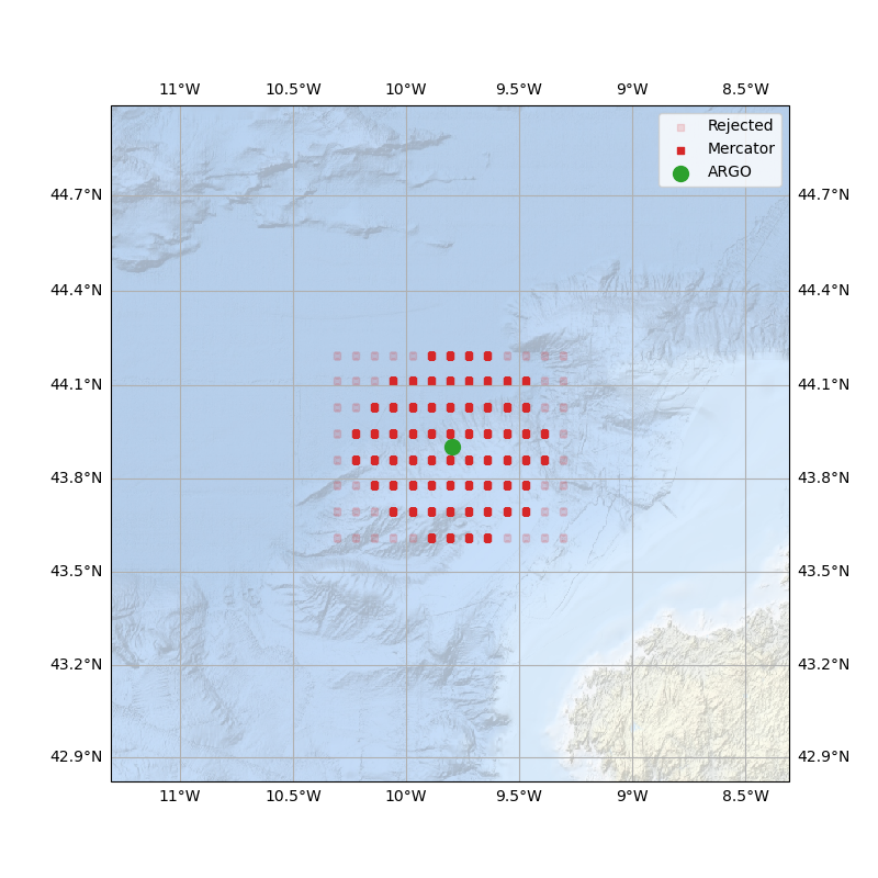
Compare Mercator and ARGO

Let’s plot the situation.

pmerc = ccrs.Mercator()
pcar = ccrs.PlateCarree()
fig, ax = plt.subplots(subplot_kw={"projection": pmerc}, figsize=(8, 8))
ax.set_extent(xgeo.get_extent(ds_merc, margin=1, square=True))
ax.gridlines(draw_labels=True)
ax.add_wms("https://ows.emodnet-bathymetry.eu/wms", "emodnet:mean_atlas_land", alpha=0.5)
kws = dict(c="C3", s=15, marker="s", transform=pcar)
ax.scatter(ds_merc_ens_rect.lon, ds_merc_ens_rect.lat, label="Rejected", alpha=0.15, **kws)
ax.scatter(ds_merc_ens.lon, ds_merc_ens.lat, label='Mercator', **kws)
ax.scatter(ds_argo_prof.lon, ds_argo_prof.lat, s=100, c="C2", transform=pcar, label='ARGO')
plt.legend()

<matplotlib.legend.Legend object at 0x759690daa7b0>

We used the xoa.geo.get_extent() to compute a square geographical extent based on the coordinates of a dataset with an added margin.

Now interpolate Mercator onto ARGO time and position for both the ensemble and the reference profile. All interpolations can be performed with the interp() method since we are dealing with axis (1D) coordinates.

ds_merc_ens = ds_merc_ens.interp(time=ds_argo_prof.time.values)
ds_merc_ens_std = ds_merc_ens.std("member")
ds_merc_prof = ds_merc.interp(time=ds_argo_prof.time, lon=ds_argo_prof.lon, lat=ds_argo_prof.lat)

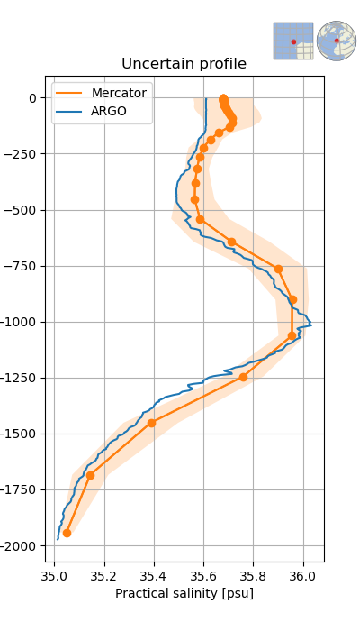
We plot now the model, its simulated uncertainty and the observations.

plt.figure(figsize=(4, 7))
plt.fill_betweenx(
    ds_merc_prof.sal.depth,
    ds_merc_prof.sal - 1.96 * ds_merc_ens_std.sal,
    ds_merc_prof.sal + 1.96 * ds_merc_ens_std.sal,
    fc="C1",
    alpha=0.2,
)
ds_merc_prof.sal.plot(y="depth", color="C1", label="Mercator")
plt.plot(ds_merc_prof.sal.values, ds_merc_prof.depth, "o-", color="C1")
ds_argo_prof.sal.plot(y="depth", label="ARGO", color="C0")
plt.title("Uncertain profile")
plt.legend()
xplot.plot_double_minimap(
    ds_argo_prof,
    regional_ax="left",
    global_ax=(0.88, 0.88, 0.11),
)

(<GeoAxes: >, <GeoAxes: >)

Therefore, if we accept an uncertainty in the positioning of the ocean structure in the model, it differences with (assimilated) observations become acceptables.

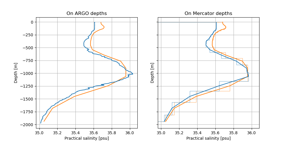
As you can see on the previous figures, the ARGO profiles come with a very high vertical resolution at all depths, whereas the model comes with a crude vertical resolution far from the surface. Each model thermodynamical model value is representative of the cube that defines its XYZ cell. This means that despite the model does simulate the small scale variability, the cell average may be accurate. So we propose here to perform comparisons in the model and the observational spaces. We use the function xoa.regrid.regrid1d() that supports the linear (linear method) interpolation to higher resolutions and the cell averaging (cellave method) to lower resolutions.

sal_merc_ens_o = xregrid.regrid1d(ds_merc_ens.sal, ds_argo_prof.depth, method="linear")
sal_merc_prof_o = xregrid.regrid1d(ds_merc_prof.sal, ds_argo_prof.depth, method="linear")
sal_argo_prof_m = xregrid.regrid1d(ds_argo_prof.sal, ds_merc_prof.depth, method="cellave")
merc_prof_edges = xgrid.get_edges(ds_merc_prof.depth, "depth")

Let’s plot them.

fig, axes = plt.subplots(ncols=2, sharex=True, sharey=True, figsize=(10, 5))
sal_merc_prof_o.plot(y="depth", color="C1", label="Mercator", ax=axes[0])
ds_argo_prof.sal.plot(y="depth", label="ARGO", color="C0", ax=axes[0])
axes[0].set_title("On ARGO depths")
axis = axes[0].axis()
ds_merc_prof.sal.plot(y="depth", color="C1", label="Mercator", ax=axes[1])
plt.stairs(ds_merc_prof.sal, merc_prof_edges, orientation="horizontal", color="C1", lw=0.5)
sal_argo_prof_m.plot(y="depth", label="ARGO", color="C0", ax=axes[1])
plt.stairs(sal_argo_prof_m, merc_prof_edges, orientation="horizontal", color="C0", lw=0.5)
axes[1].set_title("On Mercator depths")
axes[1].axis(axis)

(np.float64(34.96304988861084), np.float64(36.083950996398926), np.float64(-2072.132029431184), np.float64(92.43771385860644))

These plots show that the model is too haline, except at the mediterranean water depth where the model is very close to the observations once an appropriate vertical regridding is performed. However, the vertical resolution is not sufficient enough to simulate the maximum of salinity.