Note
Go to the end to download the full example code. or to run this example in your browser via Binder
Interpolate a meridional section of CROCO outputs to regular depths#
In this notebook, we show:
how to compute the depths from s-coordinates,
how to easily find the name of variables and coordinates,
how to interpolate a 3D field with varying depths to regular depths,
how to compute the mixed layer depth from temperature.
Initialisations#
Import needed modules.
import numpy as np
import xarray as xr
import matplotlib.pyplot as plt
import cmocean
import xoa
from xoa.regrid import regrid1d
from xoa.thermdyn import mixed_layer_depth
import xoa.cf as xcf

xr.set_options(display_style="text")
<xarray.core.options.set_options object at 0x7d7e72a68440>
Register the xarray.Dataset.decode_sigma() callable accessor.
xoa.register_accessors(decode_sigma=True)
The xoa accessor is also registered by default, and give access to most of the fonctionalities of the other accessors.
Register the internal CROCO naming specifications
croco_cfg_file = xoa.get_cf_config_file("croco")
print(croco_cfg_file)
xcf.register_cf_specs(croco_cfg_file)
/home/docs/checkouts/readthedocs.org/user_builds/xoa/conda/stable/lib/python3.13/site-packages/xoa/cf_configs/croco.cfg
You can provide your own configuration file.
In this way, the xoa.cf module will recognise the
CROCO netcdf names.
It would be equivalent to force loading name specs with
xoa.cf.set_cf_specs(xoa.get_cf_config_file(“croco”)).
Read the model#
This sample is a meridional extraction of a full 3D CROCO output.
sample_file = xoa.get_data_sample("croco.south-africa.meridional.nc")
print(sample_file)
ds = xr.open_dataset(sample_file)
print(ds)
/home/docs/checkouts/readthedocs.org/user_builds/xoa/conda/stable/lib/python3.13/site-packages/xoa/data_samples/croco.south-africa.meridional.nc
<xarray.Dataset> Size: 48kB
Dimensions:     (time: 1, s_w: 33, eta_rho: 56, xi_rho: 1, s_rho: 32,
                 eta_v: 55, xi_u: 1, auxil: 4)
Coordinates: (12/13)
  * eta_rho     (eta_rho) float32 224B 6.0 7.0 8.0 9.0 ... 58.0 59.0 60.0 61.0
  * eta_v       (eta_v) float32 220B 6.5 7.5 8.5 9.5 ... 57.5 58.5 59.5 60.5
    lat_rho     (eta_rho, xi_rho) float32 224B ...
    lat_u       (eta_rho, xi_u) float32 224B ...
    lat_v       (eta_v, xi_rho) float32 220B ...
    lon_rho     (eta_rho, xi_rho) float32 224B ...
    ...          ...
    lon_v       (eta_v, xi_rho) float32 220B ...
  * s_rho       (s_rho) float32 128B -0.9844 -0.9531 ... -0.04688 -0.01562
  * s_w         (s_w) float32 132B -1.0 -0.9688 -0.9375 ... -0.0625 -0.03125 0.0
  * time        (time) float64 8B 2.592e+06
  * xi_rho      (xi_rho) float32 4B 131.0
  * xi_u        (xi_u) float32 4B 131.5
Dimensions without coordinates: auxil
Data variables: (12/23)
    AKt         (time, s_w, eta_rho, xi_rho) float32 7kB ...
    Cs_r        (s_rho) float32 128B ...
    Cs_w        (s_w) float32 132B ...
    Vtransform  float32 4B ...
    angle       (eta_rho, xi_rho) float32 224B ...
    el          float32 4B ...
    ...          ...
    time_step   (time, auxil) int32 16B ...
    u           (time, s_rho, eta_rho, xi_u) float32 7kB ...
    v           (time, s_rho, eta_v, xi_rho) float32 7kB ...
    w           (time, s_rho, eta_rho, xi_rho) float32 7kB ...
    xl          float32 4B ...
    zeta        (time, eta_rho, xi_rho) float32 224B ...
Attributes: (12/57)
    type:           ROMS history file
    title:          BENGUELA TEST MODEL
    date:
    rst_file:       CROCO_FILES/croco_rst.nc
    his_file:       CROCO_FILES/croco_his.nc
    avg_file:       CROCO_FILES/croco_avg.nc
    ...             ...
    v_sponge:       0.0
    sponge_expl:    Sponge parameters : extent (m) & viscosity (m2.s-1)
    SRCS:           main.F step.F read_inp.F timers_roms.F init_scalars.F ini...
    CPP-options:    REGIONAL BENGUELA_VHR MPI OBC_EAST OBC_WEST OBC_NORTH OBC...
    history:        Tue Mar 31 16:26:24 2020: ncks -O -d time,30 -d xi_rho,13...
    NCO:            4.4.2
Compute depths from s-coordinates#
Decode the dataset according to the CF conventions:
Find sigma terms
Compute depths
Assign depths as coordinates
Note that the xarray.Dataset.decode_sigma() callable accessor
calls the xoa.sigma.decode_cf_sigma() function.
<xarray.DataArray 'depth' (time: 1, s_rho: 32, eta_rho: 56, xi_rho: 1)> Size: 14kB
array([[[[-4.47877094e+03],
         [-4.45341996e+03],
         [-4.43332677e+03],
         ...,
         [-7.38942261e+01],
         [-7.34145126e+01],
         [-7.34091339e+01]],

        [[-4.10998823e+03],
         [-4.08677665e+03],
         [-4.06837926e+03],
         ...,
         [-7.04949875e+01],
         [-7.00423355e+01],
         [-7.00372620e+01]],

        [[-3.70399824e+03],
         [-3.68314555e+03],
         [-3.66661754e+03],
         ...,
...
         ...,
         [-4.29529285e+00],
         [-4.27484226e+00],
         [-4.27461290e+00]],

        [[-1.00794917e+01],
         [-1.00480584e+01],
         [-1.00177860e+01],
         ...,
         [-2.57388449e+00],
         [-2.56165075e+00],
         [-2.56151366e+00]],

        [[-3.17876252e+00],
         [-3.15406689e+00],
         [-3.12913607e+00],
         ...,
         [-8.56902122e-01],
         [-8.52836072e-01],
         [-8.52790475e-01]]]], shape=(1, 32, 56, 1))
Coordinates:
  * eta_rho  (eta_rho) float32 224B 6.0 7.0 8.0 9.0 10.0 ... 58.0 59.0 60.0 61.0
    lat_rho  (eta_rho, xi_rho) float32 224B -37.67 -37.61 ... -34.03 -33.96
    lon_rho  (eta_rho, xi_rho) float32 224B 18.83 18.83 18.83 ... 18.83 18.83
  * s_rho    (s_rho) float32 128B -0.9844 -0.9531 -0.9219 ... -0.04688 -0.01562
  * time     (time) float64 8B 2.592e+06
  * xi_rho   (xi_rho) float32 4B 131.0
    depth    (time, s_rho, eta_rho, xi_rho) float64 14kB -4.479e+03 ... -0.8528
Attributes:
    axis:           Z
    long_name:      Depth
    standard_name:  ocean_layer_depth
    units:          m
Find coordinate names from CF conventions#
The depth was assigned as coordinates at the previous stage.
We use the xoa accessor to easily access the temperature, latitude and depth arrays.
The default configuration exposes shortcuts for some variables and coordinates
as shown in accessors.
temp = ds.xoa.temp.squeeze()
temp = temp.where(temp != 0)  # convert zeros to nans
lat_name = temp.xoa.lat.name
Interpolate at regular depths#
We interpolate the temperature array from irregular to regular depths.
Let’s create the output depths.
depth = xr.DataArray(
    np.linspace(ds.depth.values.min(), ds.depth.values.max(), 1000), name="depth", dims="depth"
)
Let’s interpolate the temperature.
Compute the mixed layer depths#
The mixed layer depths are computed here as the depth at which the temperature
is deltatemp lower than the surface temperature,
thanks to the xoa.thermdyn.mixed_layer_depth() function.
Plots#
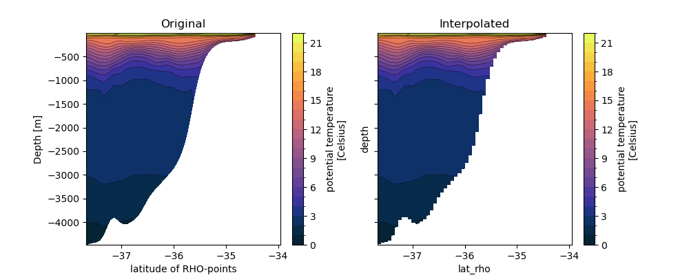
Plot the full section.
fig, axs = plt.subplots(ncols=2, sharex=True, sharey=True, figsize=(10, 4))
kw = dict(levels=np.arange(0, 23))
temp.plot.contourf(lat_name, "depth", cmap="cmo.thermal", ax=axs[0], **kw)
temp.plot.contour(lat_name, "depth", colors='k', linewidths=0.3, ax=axs[0], **kw)
tempz.plot.contourf(lat_name, "depth", cmap="cmo.thermal", ax=axs[1], **kw)
tempz.plot.contour(lat_name, "depth", colors='k', linewidths=0.3, ax=axs[1], **kw)
axs[0].set_title("Original")
axs[1].set_title("Interpolated")
Text(0.5, 1.0, 'Interpolated')
Plot a zoom near the surface and add the mixed layer depth isoline.
fig, axs = plt.subplots(ncols=2, sharex=True, sharey=True, figsize=(10, 3))
kw = dict(levels=np.arange(0, 23))
temp.plot.contourf(lat_name, "depth", cmap="cmo.thermal", ax=axs[0], **kw)
temp.plot.contour(lat_name, "depth", colors='k', linewidths=0.3, ax=axs[0], **kw)
mld.plot.line(x=lat_name, color="k", linewidth=2, linestyle="--", ax=axs[0])
tempz.plot.contourf(lat_name, "depth", cmap="cmo.thermal", ax=axs[1], **kw)
tempz.plot.contour(lat_name, "depth", colors='k', linewidths=0.3, ax=axs[1], **kw)
mldz.plot.line(x=lat_name, color="k", linewidth=2, linestyle="--", ax=axs[1])
axs[0].set_ylim(-300, 0)
axs[0].set_title("Original")
axs[1].set_title("Interpolated")
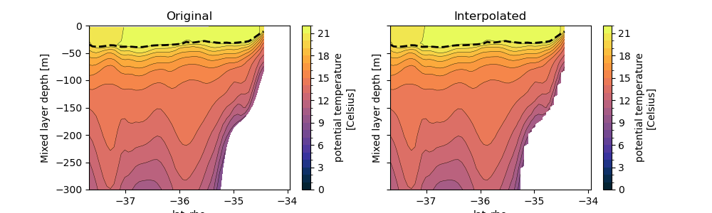
Text(0.5, 1.0, 'Interpolated')
Et voilà!
Total running time of the script: (0 minutes 6.608 seconds)