Compare Hycom3d with a GDP drifter

In this notebook, we show :

• how to decode dataset so that it is easy to access generic coordinates and variables,

• how to compute depths from layer thicknesses,

• how to interpolate currents from U and V positions to T position on an arakawa C grid,

• how to perform a 4D interpolation with a variable depth coordinate to random positions,

• how to make an horizontal slice of a 4D variable with a variable depth coordinate.

Initialisations

import numpy as np
import pandas as pd
import xarray as xr
import matplotlib.pyplot as plt
import cartopy.crs as ccrs
import xoa
from xoa.grid import dz2depth, shift
from xoa.regrid import grid2loc, regrid1d
import xoa.cf as xcf
import xoa.geo as xgeo
from xoa.plot import plot_flow, plot_double_minimap

xr.set_options(display_style="text")

<xarray.core.options.set_options object at 0x7d7e5f8b9810>

Register the xoa accessors:

xoa.register_accessors()

Set the internal Hycom naming specifications as the current ones

hycom_cfg_file = xoa.get_cf_config_file("hycom")
print(hycom_cfg_file)
xcf.set_cf_specs(hycom_cfg_file)

/home/docs/checkouts/readthedocs.org/user_builds/xoa/conda/stable/lib/python3.13/site-packages/xoa/cf_configs/hycom.cfg

<xoa.cf.set_cf_specs object at 0x7d7e69e90980>

Note that, since this file is internal, you can do it simply with:

xcf.set_cf_specs("hycom")

Here is what these CF specifications contain

with open(hycom_cfg_file) as f:
    print(f.read())

[register]
name=hycom

    [[attrs]]
    nsigma = "[0-9]?"

[sglocator]
name_format="{root}_{loc}"
valid_locations=u,v

[vertical]
positive=down
type=dz

[data_vars]

    [[u]]
    loc=u
        [[[add_coords_loc]]]
        lon=True
        lat=True
        x=True
        y=True

    [[v]]
    loc=v
        [[[add_coords_loc]]]
        lon=True
        lat=True
        x=True
        y=True

    [[bathy]]
    name=bathymetry
    add_loc=True

    [[dz]]
    name=h

[coords]

    [[x]]
    name=X

    [[y]]
    name=Y

    [[z]]
    name=lev

Note that most of these specifications are not needed to decode the dataset, i.e to find known variables and coordinates, since the default specifications help for that.

Read and decode the datasets

Hycom velocities

U and V are stored in separate files at U and V locations on the Hycom Arakawa C-Grid. We choose to rename the dataset contents so that we can use generic names to access it. We call for that the decode() accessor method. Note that the staggered grid location is automatically appended to horizontal coordinates and dimensions of the U and V velocity components since they are placed at U and V locations. This prevent any conflict with the bathymetry and layer thickness horizontal coordinates and dimensions, which point to the T location.

U velocity component

u_hycom = xoa.open_data_sample("hycom.gdp.u.nc").xoa.decode().u.squeeze(drop=True)
print(u_hycom)

<xarray.DataArray 'u' (time: 50, z: 6, y_u: 11, x_u: 13)> Size: 172kB
[42900 values with dtype=float32]
Coordinates:
    lon_u    (y_u, x_u) float32 572B ...
    lat_u    (y_u, x_u) float32 572B ...
  * z        (z) int32 24B 1 2 3 4 5 6
  * time     (time) datetime64[ns] 400B 2021-03-01 ... 2021-03-25T12:00:00
Dimensions without coordinates: y_u, x_u
Attributes:
    long_name:      Vitesse u
    units:          m/s
    standard_name:  sea_water_x_velocity

V velocity component

v_hycom = xoa.open_data_sample("hycom.gdp.v.nc").xoa.decode().v.squeeze(drop=True)

Layer thicknesses dataset

hycom = xoa.open_data_sample("hycom.gdp.h.nc").xoa.decode().squeeze(drop=True)
print(hycom)

<xarray.Dataset> Size: 174kB
Dimensions:  (y: 11, x: 13, z: 6, time: 50)
Coordinates:
    lon      (y, x) float32 572B ...
    lat      (y, x) float32 572B ...
  * z        (z) int32 24B 1 2 3 4 5 6
  * time     (time) datetime64[ns] 400B 2021-03-01 ... 2021-03-25T12:00:00
Dimensions without coordinates: y, x
Data variables:
    bathy    (y, x) float32 572B ...
    dz       (time, z, y, x) float32 172kB ...
Attributes: (12/26)
    history:                   Fri Apr  9 12:15:22 2021: ncrcat -d X,472,508,...
    Conventions:               COARDS
    nhybrd:                    20
    nsigma:                    19
    kapref:                    2
    hybflg:                    0
    ...                        ...
    dp00ft:                    [1.15 1.15 1.15 1.15 1.15 1.15 1.15 1.15 1.15 ...
    dp00xt:                    [21.874 21.414 21.414 13.197  7.85   3.85   4....
    ds00t:                     [3.555 3.026 3.026 1.547 0.828 0.828 0.968 0.8...
    ds00ft:                    [1.15 1.15 1.15 1.15 1.15 1.15 1.15 1.15 1.15 ...
    ds00xt:                    [21.874 21.414 21.414  7.197  3.85   3.85   4....
    nco_openmp_thread_number:  1

We now compute the depths from the layer thicknesses at the T location thanks to the xoa.grid.dz2depth() function: we integrate from a null SSH and interpolate the depth from W locations to T locations.

hycom.coords["depth"] = dz2depth(hycom.dz, centered=True)

Then we interpolate the velocity components to the T location with the xoa.grid.shift() function. The call to reloc helps removing the staggered grid location prefixes.

ut_hycom = shift(u_hycom, {"x": "left", "y": "left"}).xoa.reloc(u=False)
vt_hycom = shift(v_hycom, {"x": "left", "y": "left"}).xoa.reloc(v=False)
hycom["u"] = ut_hycom.assign_coords(**hycom.coords)
hycom["v"] = vt_hycom.assign_coords(**hycom.coords)

So, finally we obtain:

print(hycom)

<xarray.Dataset> Size: 689kB
Dimensions:  (y: 11, x: 13, z: 6, time: 50)
Coordinates:
    lon      (y, x) float32 572B ...
    lat      (y, x) float32 572B ...
  * z        (z) int32 24B 1 2 3 4 5 6
  * time     (time) datetime64[ns] 400B 2021-03-01 ... 2021-03-25T12:00:00
    depth    (time, z, y, x) float32 172kB 1.511 1.511 1.51 ... 20.09 20.06
Dimensions without coordinates: y, x
Data variables:
    bathy    (y, x) float32 572B ...
    dz       (time, z, y, x) float32 172kB 3.021 3.021 3.02 ... 5.22 5.216 5.209
    u        (time, z, y, x) float32 172kB 0.03078 0.02984 ... 0.1292 0.1364
    v        (time, z, y, x) float32 172kB 0.0497 0.07527 ... 0.0498 0.05054
Attributes: (12/26)
    history:                   Fri Apr  9 12:15:22 2021: ncrcat -d X,472,508,...
    Conventions:               COARDS
    nhybrd:                    20
    nsigma:                    19
    kapref:                    2
    hybflg:                    0
    ...                        ...
    dp00ft:                    [1.15 1.15 1.15 1.15 1.15 1.15 1.15 1.15 1.15 ...
    dp00xt:                    [21.874 21.414 21.414 13.197  7.85   3.85   4....
    ds00t:                     [3.555 3.026 3.026 1.547 0.828 0.828 0.968 0.8...
    ds00ft:                    [1.15 1.15 1.15 1.15 1.15 1.15 1.15 1.15 1.15 ...
    ds00xt:                    [21.874 21.414 21.414  7.197  3.85   3.85   4....
    nco_openmp_thread_number:  1

GDP drifter

The drifter comes as a csv file and we read it as pandas.DataFrame instance.

csv_name = xoa.get_data_sample("gdp-6203641.csv")
drifter = pd.read_csv(
    csv_name, header=0, skiprows=[1], parse_dates=[0], index_col=0, usecols=[2, 3, 4, 5, 6, 7]
)

Since the sampling is not that nice, we resample it to 3-hour intervals.

drifter = drifter.resample("3h").mean()

We switch to default naming conventions for the drifter.

xcf.set_cf_specs("default")

<xoa.cf.set_cf_specs object at 0x7d7e5f8ba710>

We convert it to and xarray.Dataset, fix the time coordinate and decode it.

drifter = drifter.to_xarray().assign_coords(time=drifter.index.values).xoa.decode()

We drop missing values.

drifter = drifter.where(~drifter.lon.isnull() & ~drifter.lat.isnull(), drop=True)

We add a constant depth of 15 m.

drifter.coords["depth"] = drifter.lon * 0 + 15

Here is what we obtain.

print(drifter)

<xarray.Dataset> Size: 9kB
Dimensions:  (time: 159)
Coordinates:
    lat      (time) float64 1kB 44.68 44.72 44.72 44.72 ... 44.72 44.71 44.71
    lon      (time) float64 1kB -2.544 -2.583 -2.592 ... -2.523 -2.514 -2.505
  * time     (time) datetime64[ns] 1kB 2021-03-03T18:00:00 ... 2021-03-24T09:...
    depth    (time) float64 1kB 15.0 15.0 15.0 15.0 15.0 ... 15.0 15.0 15.0 15.0
Data variables:
    sst      (time) float64 1kB 13.09 12.79 12.77 12.78 ... 12.56 12.53 12.61
    slp      (time) float64 1kB 1.027e+03 1.024e+03 ... 1.025e+03 1.026e+03
    lon360   (time) float64 1kB 357.5 357.4 357.4 357.4 ... 357.5 357.5 357.5

Compute and interpolate velocities

We compute the drifter velocity components

drifter["u"] = (
    drifter.lon.differentiate("time", datetime_unit="s") * xgeo.EARTH_RADIUS * np.pi / 180
)
drifter["u"] *= np.cos(np.radians(drifter.lat.values))
drifter["v"] = (
    drifter.lat.differentiate("time", datetime_unit="s") * xgeo.EARTH_RADIUS * np.pi / 180
)

We make a 4D linear interpolation the Hycom velocity to the drifter positions with xoa.regrid.grid2loc().

uloc = grid2loc(hycom["u"], drifter)
vloc = grid2loc(hycom["v"], drifter)

Instead of just showing the velocities along the drifter positions, we can plot the mean model velocities over the same period as a background. So we interpolate them at 15 m with xoa.regrid.regrid1d() and compute a time average.

d15 = xr.DataArray([15.0], dims="depth", name="depth")
uh15 = regrid1d(hycom["u"], d15).squeeze(drop=True).mean(dim="time")
vh15 = regrid1d(hycom["v"], d15).squeeze(drop=True).mean(dim="time")

Plot

The geographic extent is easily computed with the xoa.geo.get_extent() function. The background currents are plotted with the xoa.plot.plot_flow() function.

pmerc = ccrs.Mercator()
pcarr = ccrs.PlateCarree()
fig, ax = plt.subplots(figsize=(8, 7), subplot_kw={"facecolor": "teal", "projection": pmerc})
plt.subplots_adjust(right=0.85)
ax.gridlines(draw_labels=True, dms=True)
ax.set_extent(xgeo.get_extent(uh15))
kwqv = dict(scale_units="dots", scale=0.1 / 20, units="dots", transform=pcarr)
plot_flow(uh15, vh15, axes=ax, transform=pcarr, color="w", alpha=(0.3, 1), linewidth=0.6)
qv = ax.quiver(
    uloc.lon.values,
    uloc.lat.values,
    uloc.values,
    vloc.values,
    color="w",
    width=2,
    label="Model",
    **kwqv,
)
ax.plot(drifter.lon.values, drifter.lat.values, '-', color="C1", transform=pcarr, lw=0.5)
ax.quiver(
    drifter.lon.values,
    drifter.lat.values,
    drifter.u.values,
    drifter.v.values,
    color="C1",
    label="Drifter",
    width=2,
    **kwqv,
)
plt.quiverkey(qv, 0.1, 1.06, 0.1, r"0.1 $m\,s^{-1}$", color="k", alpha=1, labelpos="E")
plt.legend()
plot_double_minimap(drifter)

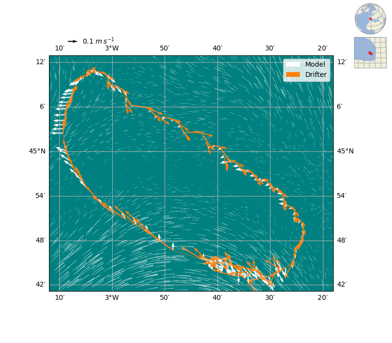
(<GeoAxes: >, <GeoAxes: >)

The discrepancies between the lagrangian and mean eulerian currents highlight the variability due to the mesocale activity. The differences between the observed and modeled currents are partly due to the lack of data assimilation in the model.